Newer insights have unmasked established concepts as unreliable in certain cases. As a reference, I take the worst type of optimizer - Markowitz' concept of diversification. But also in times where the market shifts into new regimes established models do not work properly - Black vs. Bachelier revisited.
Thank You for Reading

Statistics tells us that in 2013 about 45.000 pages were read in this blog (from about 110.000 since mid 2009).
This is because we provided even more views behind the curtain (Mathematics Wednesday and Physics Friday) and try now to share ideas every working day.
Not surprisingly, the number of page entries are led by MATHEMATICS and the post hit list shows the interest in the background and foreground of computational finance, the UnRisk Financial Language and advanced risk management approaches.
The most popular posts this year were not the best ones?
Like in music, movies, restaurants, … "best" is rarely the same as "popular", but this year I find an interesting correlation between both.
2013 Hit List
Skateboarding and Computational Finance
Hows, Whys and Wherefores of FEM in Quant Finance (II)
Extreme Vasicek Examples The World was (not) Waiting For
Black vs Bachelier Revisited
Setting Boundary Conditions That You Don't Know
Flakes of Artificial Graphene in Magnetic Fields
The Big Joke of Big Data
Should Quants Learn More About Machine Learning?
CVA/FVA/DVA - Fairer Pricing or Accounting VOODOO
Dupire or Not Dupire? Is this a Question?
In Agenda 2014 we have outlined what our focus will be next year: package and disseminate know how. We tried to compile our purpose and passion into one word: quantsourcing
We wish You a Prosperous 2014!
Picture from sehfelder
Not a Christmas Story: Guide Stars
Recently, I started to write about Adaptive Optics in Achievements 2013. The basic idea in Adaptive optics is to calibrate the deformable mirror in such a way that a known star gives a sharp image.
SCAO: Single Conjugate Adaptive Optics
If the astronomers know a true star (a natural guide star) that is close to (or: in the) observation area, then this star can be used for derforming the mirror.

Different types of wavefront sensors are in use: In Shack–Hartmann SCAO systems the wavefront sensor is an array of lenslets that measures the average gradient (slopes) of the phase over each subaperture in the pupil plane.
MCAO and MOAO: Increasing the angle to be viewed.
The disadvantage of SCAO systems is the narrow field of view (typically less than 1 arc minute). Multi conjugate adaptive optic systems (MCAO) and multi object adaptive optics systems (MOAO)use artificial laser guide stars or combinations of laser guide stars and natural guidestars to increase the angle of view to several arc minutes. Such laser guide stars are obtained by sendig laser beams (like in Star Wars) into the sky which are then reflected at the sodium layer that surrounds the earth at a height of about 90 km. Due to the finite distance of this sodium layer, techniques from tomography have to be applied to detect the atmospheric turbulence at different heights of the atmosphere.
A merry Christmas to all of you.
SCAO: Single Conjugate Adaptive Optics
If the astronomers know a true star (a natural guide star) that is close to (or: in the) observation area, then this star can be used for derforming the mirror.
Different types of wavefront sensors are in use: In Shack–Hartmann SCAO systems the wavefront sensor is an array of lenslets that measures the average gradient (slopes) of the phase over each subaperture in the pupil plane.
 |
| Schematic operation of a Shack Hartmann sensor. In the ideal case, the lenslets deliver a periodic image of the guide star (top). Under a perturbed wavefront, this image bcomes irregular (bottom). Source: http://www.ctio.noao.edu/~atokovin/tutorial/part3/wfs.html |
MCAO and MOAO: Increasing the angle to be viewed.
The disadvantage of SCAO systems is the narrow field of view (typically less than 1 arc minute). Multi conjugate adaptive optic systems (MCAO) and multi object adaptive optics systems (MOAO)use artificial laser guide stars or combinations of laser guide stars and natural guidestars to increase the angle of view to several arc minutes. Such laser guide stars are obtained by sendig laser beams (like in Star Wars) into the sky which are then reflected at the sodium layer that surrounds the earth at a height of about 90 km. Due to the finite distance of this sodium layer, techniques from tomography have to be applied to detect the atmospheric turbulence at different heights of the atmosphere.
A merry Christmas to all of you.
What I am really excited about - Flakes of artificial graphene in magnetic fields
Last physic's friday before holiday season - and today I will write about something which is not directly connected to finance. Me and my colleague and friend Esa from the university of Tampere will write about Flakes of artificial graphene in magnetic fields.
Artificial graphene (AG) is a man-made nanomaterial that can be constructed by arranging molecules on a metal surface or by fabricating a quantum-dot lattice in a semiconductor heterostructure. In both cases, AG resembles graphene in many ways, but it also has additional appealing features such as tunability with respect to the lattice constant, system size and geometry, and edge configuration.
Here we solve numerically the electronic states of various hexagonal AG flakes. The next picture shows our results when calculating the electron density for such a system. It is amazing how the experiment and the simulation coincidence.

What are we going to do next: In particular, we demonstrate the formation of the Dirac point as a function of the lattice size and its response to an external, perpendicular magnetic field. Secondly,we examine the complex behaviour of the energy levels as functions of both the system size and magnetic field. Eventually, we find the formation of "Hofstadter butterfly"-type patterns in the energy spectrum. I will report about our findings as soon as they are published.
What is the connection to finance: Although not obvious the numerical methods to solve equations like the Schrödinger equation extremely fast and efficient help us to improve our numerical finance codes. Algorithms and methods used in UnRisk have proofed to work also in the fields of physics and industrial mathematics for years.
Artificial graphene (AG) is a man-made nanomaterial that can be constructed by arranging molecules on a metal surface or by fabricating a quantum-dot lattice in a semiconductor heterostructure. In both cases, AG resembles graphene in many ways, but it also has additional appealing features such as tunability with respect to the lattice constant, system size and geometry, and edge configuration.
 |
| Designer Dirac fermions and topological phases in molecular graphene. Gomes et al. NATURE | VOL 483 | 15 MARCH 2012 |

What are we going to do next: In particular, we demonstrate the formation of the Dirac point as a function of the lattice size and its response to an external, perpendicular magnetic field. Secondly,we examine the complex behaviour of the energy levels as functions of both the system size and magnetic field. Eventually, we find the formation of "Hofstadter butterfly"-type patterns in the energy spectrum. I will report about our findings as soon as they are published.
What is the connection to finance: Although not obvious the numerical methods to solve equations like the Schrödinger equation extremely fast and efficient help us to improve our numerical finance codes. Algorithms and methods used in UnRisk have proofed to work also in the fields of physics and industrial mathematics for years.
Achievements 2013: Adaptive Optics
As mentioned in Telescopes and Mathematical Finance, we, together with the Industrial Mathematics Institute (Johannes Kepler Unibersität Linz) and the Radon Institute for Computational and Applied Mathematics (RICAM) of the Autrian Academy of Sciences, have been working on mathematical algorithms for Adaptive Optics for the last years. The achievements will be used in very large and extremely large ground-based telescopes.
The point spread function of a telescope describes, roughly speaking, how sharp an image can be under ideal conditions and, therefore, how well two distinct objects (think of a planet in the vicinity of a star) can be separated. When the primary mirror of a telescope gets larger, the point spread function gets closer to a delta distribution. This is the main reason for building extremely large telescopes.
The sharpness of the images is not only influenced by the point spread function but also by blurring through turbulences in the atmosphere. Adaptive optics uses deformable mirrors to correct blurred images.

If there were no atmosphere, the incoming wavefronts from a star to be observed would be parallel. The deformable mirror, optimally adjusted, corrects the perturbations. These perturbations change, more or less, continuously so that the actuator commands for the deformable mirror have to be calculated with a frequency of 500 to 3000 Hertz.
Next: SCAO, MCAO and MOAO.
 |
| Model of the European Extremely Large Telescope (E-ELT) which should go into operation in the early 2020s. Its primary mirror will have a diameter of 39 meters. Compare its size to that of the Munich football stadium. |
The sharpness of the images is not only influenced by the point spread function but also by blurring through turbulences in the atmosphere. Adaptive optics uses deformable mirrors to correct blurred images.
If there were no atmosphere, the incoming wavefronts from a star to be observed would be parallel. The deformable mirror, optimally adjusted, corrects the perturbations. These perturbations change, more or less, continuously so that the actuator commands for the deformable mirror have to be calculated with a frequency of 500 to 3000 Hertz.
Next: SCAO, MCAO and MOAO.
Why Creating Simplicity Is Not Simple
 As technology providers we are highly committed to relate to people. We want to take the interplay between our system and users and make them feel more "natural".
UnRisk Financial Language - A VaR Scenario
Recently we have written about the UnRisk Financial Language (UFL), our asset enabling quants to program in "their language". Up to now we did not give you examples but this will change today. I have chosen a Value at Risk scenario, as it makes it clearly obvious how a domain specific language can help to simplify things tremendously.
In a first step we set up the risk factors (Interest, Equity, FX, Credit) as a list. These list also contains the historical values and the information up to what extent the information will be taken account in the calculation (number of principal components).
In a first step we set up the risk factors (Interest, Equity, FX, Credit) as a list. These list also contains the historical values and the information up to what extent the information will be taken account in the calculation (number of principal components).
 |
| Setup risk factors |
With a one-liner we can set up the Monte Carlo scenarios. All necessary information, not explicitly passed will be calculated, for example the correlations between the risk factors.
 |
| Generating Monte Carlo scenarios, necessary parameters are calculated automatically from the market data. |
Now the scenarios will be applied to a single instrument. Using UnRisk Financial Language it would be of course possible to apply the scenarios to arbitrary portfolios.
 |
| With the time series command one can specify which risk factors will be applied. |
 |
| The actual market data set describes today's market data and is needed to create scenario deltas. |
 |
| We will apply the scenario deltas to a fixed rate bond. |
 |
| We calculate the scenarios deltas |
The results can be extracted easily by again providing high level commands.
 |
| Scenario Delta Values for the fixed rate bond. Additionally one can of course get out the single risk factor scenario deltas. |
The above example shows how a programmatically elaborate task can be simplified significantly by using a domain specific language like UnRisk Financial Language.
Additionally to the high level UFL we think it is necessary to provide the information how things are calculated at the bottom. Therefore we have set up the UnRisk Academy and have written the Workout in Computational Finance.
Brownian Motion Playground
In our previous physics Friday posts we discussed Brownian motion, starting with some historical anecdotes and showing where in nature Brownian notion occurs.
Today's post delivers a little app to play with and to get a feeling for the properties of Brownian motion with a drift.
You can download the app here. The Wolfram CDF player to run the app can be downloaded here.
Today's post delivers a little app to play with and to get a feeling for the properties of Brownian motion with a drift.
 |
| Screenshot of the Brownian Motion App |
You can download the app here. The Wolfram CDF player to run the app can be downloaded here.
Quant Finance and Mechanized Intelligence - Average is Over?
I enjoy reading Tyler Cowen's Blog Marginal Revolution. His recent book is Average is Over. It is about the challenge to complement machine intelligence, greatly commented in David Brooks column Thinking for the Future .
Tempering Monte Carlo
Counting the number of magic squares of order 6 exactly, is much more complicated than those of order 4 and 5, which were discussed in Magic Squares and Algorithms for Finance.
Similar arguments to those given there show that by rotation, reflection and simultaneous intersection of rows and columns, you can obtain 192 magic squares from one arrangement of magic rows, columns and diagonals.
For the last several years, my private working horse computer (with an i7 processor) has been calculating about a trillion (10^12) magic squares of order 6, and the end is not near at all. Is there a different way to count or to estimate the number of magic squares of order 6?
Already in 1998, K. Pinn and C. Wieczerkowski (Institute for Theoretical Physics, Münster, at that time) published their paper Number of Magic Squares From Parallel Tempering Monte Carlo.
For a configuration C (a permutation of the numbers 1 thru 36), they define the "energy" E(C) to be the sum of squared residuals of row sums, colmun sums and diagonal sums compared to the magic constant 111 (for the squares of order 6). Therefore, if a configuration is magic, then its energy is 0, otherwise it is strictly positive (and greater than 2, to be more specific.)
For a positive beta, we can (at least theoretically) calculate exp ( - beta E(C)) and sum over all configurations C. With beta going to infinity, this sum converges to the number of magic squares (counting each rotation or reflection separately).
The art, and it really is art in my eyes, is now twofold:
(1) Replace the sum over all configurations by a clever Monte Carlo simulation, which becomes increasingly difficult (larger standard deviations) for larger beta, and
(2) increase the number beta to obtain better accuracy.
Details can be found in their paper.
Their estimate for the number of magic squares of order 6 is (0.17745 ± 0.00016) × 10^20 with a 99% significance.
Two of the techniques they use are extremely relevant for finance.
(1) Of course, Monte Carlo simulation and accuracy estimates are essential in valuation of derivative products.
(2) The tempering (increasing the beta) is a technique which is also essential in simulated annealing, a method from global optimization.
Similar arguments to those given there show that by rotation, reflection and simultaneous intersection of rows and columns, you can obtain 192 magic squares from one arrangement of magic rows, columns and diagonals.
For the last several years, my private working horse computer (with an i7 processor) has been calculating about a trillion (10^12) magic squares of order 6, and the end is not near at all. Is there a different way to count or to estimate the number of magic squares of order 6?
 |
| An example of a 6x6 magic square: All numbers in the diagonals are (here) between 13 and 24. |
Already in 1998, K. Pinn and C. Wieczerkowski (Institute for Theoretical Physics, Münster, at that time) published their paper Number of Magic Squares From Parallel Tempering Monte Carlo.
For a configuration C (a permutation of the numbers 1 thru 36), they define the "energy" E(C) to be the sum of squared residuals of row sums, colmun sums and diagonal sums compared to the magic constant 111 (for the squares of order 6). Therefore, if a configuration is magic, then its energy is 0, otherwise it is strictly positive (and greater than 2, to be more specific.)
For a positive beta, we can (at least theoretically) calculate exp ( - beta E(C)) and sum over all configurations C. With beta going to infinity, this sum converges to the number of magic squares (counting each rotation or reflection separately).
The art, and it really is art in my eyes, is now twofold:
(1) Replace the sum over all configurations by a clever Monte Carlo simulation, which becomes increasingly difficult (larger standard deviations) for larger beta, and
(2) increase the number beta to obtain better accuracy.
Details can be found in their paper.
Their estimate for the number of magic squares of order 6 is (0.17745 ± 0.00016) × 10^20 with a 99% significance.
Two of the techniques they use are extremely relevant for finance.
(1) Of course, Monte Carlo simulation and accuracy estimates are essential in valuation of derivative products.
(2) The tempering (increasing the beta) is a technique which is also essential in simulated annealing, a method from global optimization.
Radical Innovation - Revolution of Heroes or Heroes of Revolution?
 I like music from all directions (from John Adams to John Zorn). Who are the innovators in music?
Examples from Jazz.
What was it that so many great musicians played, say, Bebop (Dizzy Gillepie, Charly Parker, Bud Powell, Thelonious Monk, Max Roach ..), Free Jazz (Ornette Coleman, John Coltrane, Charles Mingus, Archie Shepp, Cecil Taylor, ..), Loft Jazz (Anthony Braxton, Arthur Blythe, Julius Hemphill, David Murray, Sam Rivers, …) … or those around John Zorn (improvised music, hardcore, klezmer-oriented free jazz, …)?
A coincidence of talented artists at a time? Or are artists motivated to join a revolution - and share their best work?
Quant Development - A Fractal Project Performance Model
The performance of a quant finance development project depends on the skills of the team members, their organizational interplay, the methods and tools.
The team contributions and their organizational consequences to the success of a project are usually modeled in Bell Curves (top- average- and under-performers under the law of average and standard deviation). But this does not work well for performance measurement systems, because dependencies make a project much more complex (Quants- Racers at Critical Paths).
The team contributions and their organizational consequences to the success of a project are usually modeled in Bell Curves (top- average- and under-performers under the law of average and standard deviation). But this does not work well for performance measurement systems, because dependencies make a project much more complex (Quants- Racers at Critical Paths).
Brownian Motion in 1D Structures
As mentioned in the last of my posts the main problem to observe truly one dimensional Brownian motion is the fabrication of narrow structures. In organic chemistry one important material is tetrathiafulvalene-tetracyanoquinodimethane (TTF-TCNQ)
The large planar molecules are preferentially located on top of each other, and the one dimensionality of the electronic band structure is enhanced by the directional nature of the highest molecular orbitals. With the experimental technique of NMR (Nuclear Magnetic Resonance) one can monitor the motion of the electronic spin in these one dimensional bonds [Soda et. al. J.Phy. 38,931,(1977)].
In an ideal world without perturbations one would observe a sharp delta function agh the nuclear Larmor frequency. However, perturbations generate random magnetic fields at the sites of the nucleus and lead to a broadening of the resonance line. A source of perturbation is the electronic spins which couple to the nuclear spins through hyperfine interaction and thus generating a fluctuating magnetic field (at the nucleus site) reflecting the dynamics of the electron spin motion.
Assuming the electrons perform a random walk in one dimension it can be shown using the spin-spin correlation function that the spin lattice relaxation rate for this case needs to be proportional to x=1/Sqrt(H), where H is the initial external magnetic field.
In the measurement the spin-lattice relaxation rate is measured which is then plotted versus x. There is a wide range where the relaxation rate is proportional to 1/Sqrt(H) indicating 1D diffusion of electronic spins.
 |
| Structure of TTF-TCNQ (image downloaded from http://www.intechopen.com/books/nanowires-fundamental-research/nanowires-of-molecule-based-conductors) |
In an ideal world without perturbations one would observe a sharp delta function agh the nuclear Larmor frequency. However, perturbations generate random magnetic fields at the sites of the nucleus and lead to a broadening of the resonance line. A source of perturbation is the electronic spins which couple to the nuclear spins through hyperfine interaction and thus generating a fluctuating magnetic field (at the nucleus site) reflecting the dynamics of the electron spin motion.
Assuming the electrons perform a random walk in one dimension it can be shown using the spin-spin correlation function that the spin lattice relaxation rate for this case needs to be proportional to x=1/Sqrt(H), where H is the initial external magnetic field.
In the measurement the spin-lattice relaxation rate is measured which is then plotted versus x. There is a wide range where the relaxation rate is proportional to 1/Sqrt(H) indicating 1D diffusion of electronic spins.
The New UnRisk Academy Event Blog

A common cold has killed today's mathematics wednesday post.
This is to inform you that the UnRisk Academy launched a Blog to present its courses, seminars, workouts, .. in a form that allows more detailed descriptions but keep an overview archive: UnRisk Academy Events.
5 "Don'ts" Heads of Quant Teams Should Remember

Idealism And Realism in Programming - UnRisk Financial Language

Idealism vs Realism in programming?
Idealism strives for abstraction, expressiveness, productivity, portability, …
Realism is driven by implementation, efficiency, performance, system programming, …
Observations of Brownian Motion in Nature
First systematic observations of Brownian motion in nature were made by the French physicist Jean Perrin in 1909. He recorded the position of colloidal particles suspended in a liquid every 30-50 seconds.
Note that in the picture above the straight lines are due to interpolation. Perrin noted that by shortening the observation time the paths became more ragged on even smaller scales. This was the first experimental confirmation of Einstein's theory of Brownian motion, and on diffusion in suspension. The observed Brownian motion occurred in 3D. Can we also observe 1D Brownian motion in nature?
The main problem to observe 1D Brownian motion in nature is the fabrication of structures that which are narrow enough , so that the microscopic diffusion process becomes 1d. This means that the structures need to be of the size of the diffusing particles.
The first branch of science to achieve this goal has been organic chemistry. Starting from around the mid 1960s there has been put a considerable amount of work on low dimensional materials conducting electric current. Reason was the prediction of a theory that superconductivity would be achievable at room temperature in quasi 1D structures. Although this aim has not been achieved, a lot if interesting physics has been discovered on the way. Next week we will discuss the case of 1D Brownian motion in a synthesised 1D organic conductor.
 |
| The irregular motion of suspended particles in a solution as recorded by Jean Perrin (http://www.mpiwg-berlin.mpg.de/en/research/projects/NWGII_BiggBMcorr - Charlotte Bigg) |
The main problem to observe 1D Brownian motion in nature is the fabrication of structures that which are narrow enough , so that the microscopic diffusion process becomes 1d. This means that the structures need to be of the size of the diffusing particles.
The first branch of science to achieve this goal has been organic chemistry. Starting from around the mid 1960s there has been put a considerable amount of work on low dimensional materials conducting electric current. Reason was the prediction of a theory that superconductivity would be achievable at room temperature in quasi 1D structures. Although this aim has not been achieved, a lot if interesting physics has been discovered on the way. Next week we will discuss the case of 1D Brownian motion in a synthesised 1D organic conductor.
The UnRisk Financial Language and the Babylonian Tower

Magic Squares and Algorithms for Finance
In my recent post Equation Solving for Kids, I introduced magic squares and reported the number of magic squares of the order 4 to be 880. The first computer program I wrote for calculating this number was in interpretted Basic on a Sharp MZ80A (with 32 kByte memory) in the early 1980s, and it took about 3 days to calculate them. On contemporary hardware, compiled versions need less than1 second.
Magic squares of order 5
The magic sum of the order 5 squares is 65, and there are 12 equations to be satisfied (5 rows, 5 columns, 2 diagonals). One of these equations is redundant, so there are 14 free entries. If you set , e.g., the entries marked by "x", you can calculate the remaining entries explicitly.

All these "x"-es must be integers between 1 and 25, and they must be different. How many possibilities are there? There are Binomial (25, 14) pssibilities to choose 14 numbers out of 25. As position plays a role, this has to be multiplied by Factorial(14). Thus, we obtain 388588515194880000 possibilities to set the "x" entries. Solving the system for the empty cells, does not necessarily yield a magic square which additionally has to satisfy that all 25 entries are different and lie between 1 and 25. Obviously, if you iterate the "x"-es in 14 nested loops, you should calculate dependent entries as soon as possible and jump out of the loop if the magic conditions cannot be satisfied any more.
Implementing such an algorithm, you can find out that the number of magic squares of order 5 is 2202441792.
Reordering Rows and Columns
When you know that the following square is magic,

you can interchange rows 1 and 2 and rows 4 and 4, respectively, and the interchange columns 1 and 2 and columns 4 and 5, to obtain
 which is again magic. Similarly, you could also interchange row 2 and 4, and columns 2 and 4.
Following these ideas, you can rearrange (by rotations, reflections and rows/colums interchanging) any magic square of order 5 in such a way that the smallest off-center diagonal element will be located in position (1,1) (8 possibilities), that a15 < a51 (by possible reflection, 2 possibilities) and that a22 < a44 (2 possibilities).
This reduces the effort to be taken by a factor 32. Additional computing time can be saved by taking into account that the square (26 - aij) is also magic. Be careful with double-counting when a33=13.
Not knowing the work of Richard Schroeppel (1973), I calculated the number of order 5 squares in the early 1990s on a MicroVax 3500 (see below, with 8MB of memory). My Fortran code took about 8 hours of CPU time.

Lessons learned for algorithm development
The above ideas to reduce the number of candidates have several similarities in Monte Carlo simulation for finance applications: From my point of view, interchanging rows and columns is related to antithetic variables in Monte Carlo simulation.
Exiting loops as soon as possible (magic squares) is somehow related to rejecting paths of Monte Carlo simulation in risk management, e.g., when you kno in advance that the path considered will not end in extreme percentiles.
Next week: The other way round: Monte Carlo simulation and magic squares.
Magic squares of order 5
The magic sum of the order 5 squares is 65, and there are 12 equations to be satisfied (5 rows, 5 columns, 2 diagonals). One of these equations is redundant, so there are 14 free entries. If you set , e.g., the entries marked by "x", you can calculate the remaining entries explicitly.
Implementing such an algorithm, you can find out that the number of magic squares of order 5 is 2202441792.
Reordering Rows and Columns
When you know that the following square is magic,


Following these ideas, you can rearrange (by rotations, reflections and rows/colums interchanging) any magic square of order 5 in such a way that the smallest off-center diagonal element will be located in position (1,1) (8 possibilities), that a15 < a51 (by possible reflection, 2 possibilities) and that a22 < a44 (2 possibilities).
This reduces the effort to be taken by a factor 32. Additional computing time can be saved by taking into account that the square (26 - aij) is also magic. Be careful with double-counting when a33=13.
Not knowing the work of Richard Schroeppel (1973), I calculated the number of order 5 squares in the early 1990s on a MicroVax 3500 (see below, with 8MB of memory). My Fortran code took about 8 hours of CPU time.

Lessons learned for algorithm development
The above ideas to reduce the number of candidates have several similarities in Monte Carlo simulation for finance applications: From my point of view, interchanging rows and columns is related to antithetic variables in Monte Carlo simulation.
Exiting loops as soon as possible (magic squares) is somehow related to rejecting paths of Monte Carlo simulation in risk management, e.g., when you kno in advance that the path considered will not end in extreme percentiles.
Next week: The other way round: Monte Carlo simulation and magic squares.
With UnRisk Financial Language Quants Get Something Really Big
I am heading to the airport (to London), not able to write a post by the next wednesday. So I add one today - motivated by Stephen Wolfram's contribution - A Very Big Thing Is Coming, Wolfram Blog.
Diffusion and Osmotic Pressure
In last weeks physic's friday post we made some general remarks about diffusion and Einstein's ideas. Today we want to discuss the experimental setup in more detail.
To get access to the phenomenon of osmotic pressure consider a solution where the solute is dissolved in a concentration c in the solvent in a volume V' enclosed by a membrane. This membrane is only permeable to the solvent and not to the solute. Furthermore it is assumed to be immersed in a surrounding volume of solvent, meaning a free flow of solvent in- and out is possible. Then a pressure p induced by the solute acts on the membrane - the osmotic pressure. Within the ideal gas framework the pressure can be described as
To get access to the phenomenon of osmotic pressure consider a solution where the solute is dissolved in a concentration c in the solvent in a volume V' enclosed by a membrane. This membrane is only permeable to the solvent and not to the solute. Furthermore it is assumed to be immersed in a surrounding volume of solvent, meaning a free flow of solvent in- and out is possible. Then a pressure p induced by the solute acts on the membrane - the osmotic pressure. Within the ideal gas framework the pressure can be described as
pV'=cRT
where R is the ideal gas constant. We can justify this ansatz by assuming that in a solution the size of the solute is microscopic (atomic or molecular) resembling the idea of the ideal gas.
 |
| Sketch of the idea of osmotic pressure (picture from http://www.sparknotes.com/chemistry/solutions/colligative/section1.rhtml) |
On the other hand in a suspension the particles immersed in the fluid are macroscopic. Classical thermodynamics would suggest an osmotic pressure equal to 0. Einstein's (and some others) findings corrected this view with the statistical theory of heat which answers the question which microscopic changes are originated by the addition and removal of heat. Addition and removal of heat simply increases (decreases) the motion of the particles. As a consequence both microscopical as well as macroscopic quantities must follow the same laws of motion and of statistical mechanics. As a consequence osmotic pressure is built up both in solution and suspensions. Furthermore there is a unique expression for the diffusion constant of particles in a liquid which is proportional to 1/r. Here r is the radius of the (assumed to be spherical) particles. It is obvious that between solutions and suspensions a huge difference in the dissuasion constant may be possible, nevertheless there is no qualitative difference between them in statistical mechanics.
7 Paradigms of Modern Risk Management

Inspired by the great book Red-Blooded Risk, Aaron Brown. How to manage risk to maximize success. Requiring the understanding that risk is two-sided, dangers and opportunities are one sided. Dangers and opportunities are often not quantifiable, we have limited ability to control them. Whatever techniques you use, analyze risks, dangers and opportunities, optimize risk, arrange things that make danger and opportunity a positive contribution.
Equation Solving for Kids
When I gave my applied math lecture to the nine-year-olds (see Catastrophic Streamlines), of course I talked also about our Telescopes solution, and the need to solve systems of linear equations there.
When you talk to children about linear equations, you should not assume that this is a common phrase in their language (this may be true for grown-ups as well). For introducing system of linear equations, I used the following problem, already formulated in ancient China:
There are a number of rabbits and doves in a cage. In all, there are 35 heads and 94 feet. How many rabbits and doves are there?
The arising system of equations can be solved by guessing, and some children are quite good there; but it is also possible to introduce Gaussian elimination (in this special case) in elementry school.
More than 2 unknowns and equations
When I asked the children for examples with more than 2 unknowns, they were too shy to tell me their thoughts. However, showing them a puzzle page of a newspaper, they realized that Sudoku solving is (at least somehow) similar to solving systems of equation. And this led me to magic squares.
In my definition, a magic n x n square (a "magic square of the order n") is a square table with n rows and n columns. You have to place the numbers 1, 2, 3, ..... n^2 into the cells of table in such a way that the sum of each row, the sum of each column and the sum of each of two main diagonals is the same.
It can be shown fairly easily that there is only one solution for the order 3, the so-called Lo Shu square (China, 600 BC). All other solutions are obtained by reflection and / or rotation.
Magic squares of order 4
The order 4 is already more interesting.

When the children are told that the magic sum is 34, they can solve this system of linear equations with 8 unknowns (more or less) easily.
If you want to know the number of magic squares of order 4, this can be done by just trying all possible permutations (or intelligent versions of such a brute force algorithm) and check if the resulting square is magic. It turns out that the number of essentially different magic squares is 880.
Next week: Magic squares of order 5 and 6 and algorithmic connections to finance.
When you talk to children about linear equations, you should not assume that this is a common phrase in their language (this may be true for grown-ups as well). For introducing system of linear equations, I used the following problem, already formulated in ancient China:
There are a number of rabbits and doves in a cage. In all, there are 35 heads and 94 feet. How many rabbits and doves are there?
The arising system of equations can be solved by guessing, and some children are quite good there; but it is also possible to introduce Gaussian elimination (in this special case) in elementry school.
More than 2 unknowns and equations
When I asked the children for examples with more than 2 unknowns, they were too shy to tell me their thoughts. However, showing them a puzzle page of a newspaper, they realized that Sudoku solving is (at least somehow) similar to solving systems of equation. And this led me to magic squares.
In my definition, a magic n x n square (a "magic square of the order n") is a square table with n rows and n columns. You have to place the numbers 1, 2, 3, ..... n^2 into the cells of table in such a way that the sum of each row, the sum of each column and the sum of each of two main diagonals is the same.
It can be shown fairly easily that there is only one solution for the order 3, the so-called Lo Shu square (China, 600 BC). All other solutions are obtained by reflection and / or rotation.
 |
| Lo Shu square. Image Source: Wikimedia commons |
The order 4 is already more interesting.

When the children are told that the magic sum is 34, they can solve this system of linear equations with 8 unknowns (more or less) easily.
If you want to know the number of magic squares of order 4, this can be done by just trying all possible permutations (or intelligent versions of such a brute force algorithm) and check if the resulting square is magic. It turns out that the number of essentially different magic squares is 880.
Next week: Magic squares of order 5 and 6 and algorithmic connections to finance.
3 Benefits Working for Small Market Participants
After I have posted - UnRisk Is For Small … - I thought about the influence of this business-motivated segment selection on project qualities and team satisfaction.
UnRisk Is For Small and Medium Sized Institutions and Quant Teams
In Cleaning up finance Mark Buchanan has put a few things under
tiny rays of hope that one day we might get some regulators with real teeth to reform the financial systemFirst he refers to K. C. Griffin, CEO of Citadel, who advocates breaking up big banks
to encourage the flowering of smaller banks with competitive advantages on the local level (he mentions in particular putting caps on the size of deposits)Independent of political decisions, we have decided to make Big Systems For The Small. This is part of our brand promise, as reverse innovation and in consequence quantsourcing.
Register Now for the UnRisk Workout in Computational Finance
30-Jan-14 at BBA's Pinners Hall in London.
Quants and quant developers, join us for a one-day workout with inspiring sessions on the risky horror of model and method traps and how to avoid them. We give you full explanation of the application of advanced numerical schemes to the analytics of financial instruments and portfolios thereof.
Quants and quant developers, join us for a one-day workout with inspiring sessions on the risky horror of model and method traps and how to avoid them. We give you full explanation of the application of advanced numerical schemes to the analytics of financial instruments and portfolios thereof.
Einstein contra Thermodynamics
From todays's point of view Einstein's starting point for his work on Brownian motion is rather surprising. Classical thermodynamics implies that there is no osmotic pressure in suspensions. Einstein did not intend to explain Brownian motion, the small irregular motion of particles first observed by the Scottish botanist R. Brown under the microscope, but to show that the statistical theory of heat required the motion of particles in suspensions, and therefore both diffusion and an osmotic pressure.

Contrary to thermodynamics which only works with macroscopic state variables, the statistical theory of heat tries to answer the question which microscopic changes are originated by the addition or removal of heat. Heat is related to an irregular state of motion of the microscopic building blocks of matter , such as atoms and molecules - addition/removal of heat therefore corresponds to an increase/decrease in motion.
R. Brown (1773-1858)
Video of Brownian motion of nano particles in water (YouTube-Rutger Saly)
Contrary to thermodynamics which only works with macroscopic state variables, the statistical theory of heat tries to answer the question which microscopic changes are originated by the addition or removal of heat. Heat is related to an irregular state of motion of the microscopic building blocks of matter , such as atoms and molecules - addition/removal of heat therefore corresponds to an increase/decrease in motion.
2014 Trends - The HFT Boom Turns Into A Downturn?

Institutions have invested into HFT, in the hope of gaining a millisecond advantage over their rivals. But 2014, that will all change?!
Libor and the Negative Eigenvalue Trap
In my previous post Negative Eigenvalues in Practical Finance I gave a few examples of variance-covariance matrices that are not positive definite. One of them was using a wrong correlation ansatz in the Libor market model. What happens if you as a quant are requested to write a numerical solver for such an equation with possibly negative eigenvalues?
The model problem
We consider the following partial differential equation with initial and boundary conditions

When both eigenvalues (lambda_1, lambda_2) are positive, this is an anisotropic heat equation that can be solved numerically, e.g., by a finite difference scheme. If the Courant-Friedrichs-Levy condition (that restricts the length of the time step) is satisfied, even an explicit time-stepping scheme is stable and will converge.
All eigenvalues positive
If we set lambda_1 = 1, lambda_2 = 0.1, and take 50 grid points in every space direction and a time step of 1/10000, then we obtain at t = 1

Note the scale: The Dirichlet condition V=0 at all boundaries draws the solution towards zero.
Second eigenvalue negative
For lambda_1 = 1, lambda_2 = - 0.1, we obtain for t=0.02, 0.04, 0.06:


The solution explodes. The scale on the third plot is 10^19.
Negative eigenvalue closer to zero
Maybe the second eigenvalue was "too negative"? What happens for lambda_2 = - 0.01?
t=0.02
 t=0.04
 t=0.1
t=0.1
 t=0.2
t=0.2
 No chance to stabilize it
The reason for these oscillations does not lie in the explicit scheme but in the ill-posedness of the equation. In the Traunsee example, the instability of the backwards heat equation was analysed in more detail.
The model problem
We consider the following partial differential equation with initial and boundary conditions

 |
| Initial Condition for the model problem. |
All eigenvalues positive
If we set lambda_1 = 1, lambda_2 = 0.1, and take 50 grid points in every space direction and a time step of 1/10000, then we obtain at t = 1

Note the scale: The Dirichlet condition V=0 at all boundaries draws the solution towards zero.
Second eigenvalue negative
For lambda_1 = 1, lambda_2 = - 0.1, we obtain for t=0.02, 0.04, 0.06:


The solution explodes. The scale on the third plot is 10^19.
Negative eigenvalue closer to zero
Maybe the second eigenvalue was "too negative"? What happens for lambda_2 = - 0.01?
t=0.02


The reason for these oscillations does not lie in the explicit scheme but in the ill-posedness of the equation. In the Traunsee example, the instability of the backwards heat equation was analysed in more detail.
Quants - Distinguish Between Defensive and Profound Skeptic
I am sure, quants know that situation too well. You have got a new big idea, you share it and "ten" stand up with a wordy reply, why it will not work. Skeptics are all around.
Many skeptics are afraid of the new, want to embrace the status quo. They want that you, like they themselves, give up your dream.
Spectra of Random Correlation Matrices
What is then the spectrum of the correlation matrix and how does this effect our estimation for correlation?
This has been the question at the end of my last post - the answer to this question is known for several cases due to the work of Marcenko, Pastur [V. A. Marcenko and L. A. Pastur, Math. USSR-Sb, 1, 457-483 (1967)] and several others (see for example [Z. Burda, A. G ̈orlich, A. Jarosz and J. Jurkiewicz, Physica A, 343, 295-310 (2004)]).
Considering an empirical correlation matrix E of N assets using T data points, both very large, with q = N/T finite and the "true" correlation matrix C=, defining the Wishart ensemble. In statistics, the Wishart distribution is a generalization to multiple dimensions of the chi-squared distribution. It is part of a family of probability distributions defined over symmetric, nonnegative-definite matrix-valued random variables (“random matrices”).
Then for any choice (of course this choice needs to obey the properties a correlation matrix needs to fulfil) of C one can obtain the density of eigenvalues, at least numerically. In some cases the density of the eigenvalues can be calculated analytically, so for C=I.

But are the results correct in every case ? - What will happen if we consider a matrix with one large eigenvalue, separated from the "sea", the rest of the eigenvalues form. It has been shown, that the statistics of this isolated eigenvalue is Gaussian. So the Marcenko-Pastur results describe only continuous parts of the spectrum but do not apply to isolated eigenvalues.

This has been the question at the end of my last post - the answer to this question is known for several cases due to the work of Marcenko, Pastur [V. A. Marcenko and L. A. Pastur, Math. USSR-Sb, 1, 457-483 (1967)] and several others (see for example [Z. Burda, A. G ̈orlich, A. Jarosz and J. Jurkiewicz, Physica A, 343, 295-310 (2004)]).
Considering an empirical correlation matrix E of N assets using T data points, both very large, with q = N/T finite and the "true" correlation matrix C=
Then for any choice (of course this choice needs to obey the properties a correlation matrix needs to fulfil) of C one can obtain the density of eigenvalues, at least numerically. In some cases the density of the eigenvalues can be calculated analytically, so for C=I.
But are the results correct in every case ? - What will happen if we consider a matrix with one large eigenvalue, separated from the "sea", the rest of the eigenvalues form. It has been shown, that the statistics of this isolated eigenvalue is Gaussian. So the Marcenko-Pastur results describe only continuous parts of the spectrum but do not apply to isolated eigenvalues.
Empirical eigenvalue density for 406 stocks from the S&P 500, and fit using the MP distribution. Note the presence of one large eigenvalue corresponding to the market mode. (Picture taken from Financial Applications of Random Matrix Theory: Old Laces and New Pieces, Potters et al.)
6 Questions Quants On The Critical Path Should Ask Their Clients
In a previous post, I have given some thoughts on the situation that quants are often on the critical path of rather complex projects. And that the team members should show that they care and want to help.
Quants - Usually Racers At Critical Paths
Complex project: people are working on many activities that are dependent on others.
The project network: you have the work break down into tasks, a duration for each activity, dependencies and milestones. The longest sequence of tasks in the project network that are dependent and cannot be compressed is the Critical Path.
The project network: you have the work break down into tasks, a duration for each activity, dependencies and milestones. The longest sequence of tasks in the project network that are dependent and cannot be compressed is the Critical Path.
Negative Eigenvalues in Practical Finance
Last Wednesday, I tried to focus on possible numerical difficulties when one uses a matrix that is not positive semidefinite as a correlation matrix. But is such a case of practical relevance?
Rank defect
If correlation is estimated historically and the time series of historical prices is not long enough compared to the number of assets, then the correlation matrix cannot have full rank. Assume that the time series consists of 252 observations (business days in ine year) and the universum of assets contains 300 equities. Then at least 49 (=300 - (252-1)) eigenvalues of the historic correlation matrix are zero. Numerically, these may become slightly negative.
Another source of rank defect, say, in automated trading, may occur if the same equity is traded at two different trading desks and not recognized as being identical. This case was one of my first encounters with computational finance, some twenty years ago. In a portfolio of 146 equities, 4 of them occured twice, and the customer had troubles with the Cholesky decomposition.
Wrong ansatz matrix
In chapter 22.4. of "Volatility and Correlation - The Perfect Hedger and the Fox (2nd edition)",p.691, Riccardo Rebonato writes on a two parameter ansatz matrix for correlation in a Libor market model
".... one can show that the eigenvalues of rho_{i,j}, now defined by
rho_{i,j} = exp(-beta exp (-gamma min(T_i, T_j)) . abs(T_i - T_j))
are always all positive." Is this true?
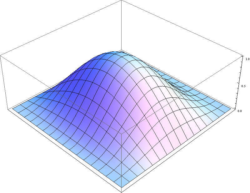
The correlation ansatz is reasonable: Libor forward rates whose starting points are close to each other are stronger correlated, and Libor foward rates in the far future are also stronger correlated. One would expect that the Libor 12m rates starting in 19 and in 20 years are much more corelated than the ones starting in 2 and in 3 years, respectively. A typical correlation surface would then have the following shape
What happens if we vary the parameters beta and gamma? Again, we use a time horizon of 30 years for annual Libor rates, and we calculate the smallest eigenvalue which should be positve.
For beta = gamma = 0.5, three eigenvalues are negative, the smallest one is -0.4, the largest one 24.6. Depending on the preferred numerical method, you can run into severe troubles.
My recommendation for working with correlation matrices is to always check (e.g. by a Cholesky decomposition) if the positive definiteness is actually fulfilled. If not, use a simpler model.
Rank defect
If correlation is estimated historically and the time series of historical prices is not long enough compared to the number of assets, then the correlation matrix cannot have full rank. Assume that the time series consists of 252 observations (business days in ine year) and the universum of assets contains 300 equities. Then at least 49 (=300 - (252-1)) eigenvalues of the historic correlation matrix are zero. Numerically, these may become slightly negative.
Another source of rank defect, say, in automated trading, may occur if the same equity is traded at two different trading desks and not recognized as being identical. This case was one of my first encounters with computational finance, some twenty years ago. In a portfolio of 146 equities, 4 of them occured twice, and the customer had troubles with the Cholesky decomposition.
Wrong ansatz matrix
In chapter 22.4. of "Volatility and Correlation - The Perfect Hedger and the Fox (2nd edition)",p.691, Riccardo Rebonato writes on a two parameter ansatz matrix for correlation in a Libor market model
".... one can show that the eigenvalues of rho_{i,j}, now defined by
rho_{i,j} = exp(-beta exp (-gamma min(T_i, T_j)) . abs(T_i - T_j))
are always all positive." Is this true?
The correlation ansatz is reasonable: Libor forward rates whose starting points are close to each other are stronger correlated, and Libor foward rates in the far future are also stronger correlated. One would expect that the Libor 12m rates starting in 19 and in 20 years are much more corelated than the ones starting in 2 and in 3 years, respectively. A typical correlation surface would then have the following shape
 |
| Correlation surface: T_i = i, i=1,..30. beta=0.05, gamma=0.1 In this specific case, the correlation matrix is indeed postive definite. |
 |
| Smallest eigenvalue, when beta and gamma vary. |
My recommendation for working with correlation matrices is to always check (e.g. by a Cholesky decomposition) if the positive definiteness is actually fulfilled. If not, use a simpler model.
Macroeconomics Discovers Finance

This weekend I have read What We've Learned From The Financial Crisis, by Justin Fox, Nov-13 issue of the HBR Magazine.
Cleaning Matrices
After last weeks overview over biases occurring in the calculation of the empirical correlation Matrix,we try to answer the question how one can "clean" matrices to avoid, at least up to a certain degree, such biases in the estimation of future risk.
In a first step we rewrite the Markowitz solution in terms of the eigenvalues l and eigenvectors V of the correlation matrix (take a look at this weeks Mathematics Wednesday, where Andreas Binder's blog post also revealed some traps in the calculation of correlation matrices).

Taking a closer look at the formula above we see, that the first term corresponds to the naive solution: one invests proportionally to the expected gains. The second term leads to a suppression of eigenvectors with l>1 and an enhancement of weights where l<1. This can lead to the situation that in the optimal Markowitz solution large weights are allocated to small eigenvalues, which may be dominated by measurement noise.
Perhaps before going on we should think over the meaning of the eigenvectors V corresponding to the large eigenvalues. The largest eigenvector corresponds to a collective market mode, whereas other large eigenvectors are sector modes. So a simple way to avoid the instability would be to project the largest eigenvalues out. This approach would lead to quite a good portfolio in terms of risk, since most of the volatility is contained in the market and sector modes.
More elaborated ways aim to use all the eigenvectors and eigenvalues but only after "cleaning them". In [L. Laloux, P. Cizeau, J.-P. Bouchaud and M. Potters, Phys. Rev. Lett. 83, 1467 (1999); L. Laloux, P. Cizeau, J.-P. Bouchaud and M. Potters, Risk 12, No. 3, 69 (1999)] it has been suggested that one should replace all low lying eigenvalues with a unique value and to keep the high eigenvalues and eigenvectors (those with the meaningful economical information - section modes)

k' is the meaningful number of sectors kept and d is chosen such that the trace of the correlation matrix is preserved. The question how to chose k' remains. In the cited publication Random Matrix Theory has been used to determine the theoretical edge of the random part of the eigenvalue distribution and to set k' such that l(k') is close to this edge.
What is then the spectrum of the correlation matrix and how does this effect our estimation for correlation. We will follow these questions in our next posts …
In a first step we rewrite the Markowitz solution in terms of the eigenvalues l and eigenvectors V of the correlation matrix (take a look at this weeks Mathematics Wednesday, where Andreas Binder's blog post also revealed some traps in the calculation of correlation matrices).
Taking a closer look at the formula above we see, that the first term corresponds to the naive solution: one invests proportionally to the expected gains. The second term leads to a suppression of eigenvectors with l>1 and an enhancement of weights where l<1. This can lead to the situation that in the optimal Markowitz solution large weights are allocated to small eigenvalues, which may be dominated by measurement noise.
Perhaps before going on we should think over the meaning of the eigenvectors V corresponding to the large eigenvalues. The largest eigenvector corresponds to a collective market mode, whereas other large eigenvectors are sector modes. So a simple way to avoid the instability would be to project the largest eigenvalues out. This approach would lead to quite a good portfolio in terms of risk, since most of the volatility is contained in the market and sector modes.
More elaborated ways aim to use all the eigenvectors and eigenvalues but only after "cleaning them". In [L. Laloux, P. Cizeau, J.-P. Bouchaud and M. Potters, Phys. Rev. Lett. 83, 1467 (1999); L. Laloux, P. Cizeau, J.-P. Bouchaud and M. Potters, Risk 12, No. 3, 69 (1999)] it has been suggested that one should replace all low lying eigenvalues with a unique value and to keep the high eigenvalues and eigenvectors (those with the meaningful economical information - section modes)
k' is the meaningful number of sectors kept and d is chosen such that the trace of the correlation matrix is preserved. The question how to chose k' remains. In the cited publication Random Matrix Theory has been used to determine the theoretical edge of the random part of the eigenvalue distribution and to set k' such that l(k') is close to this edge.
What is then the spectrum of the correlation matrix and how does this effect our estimation for correlation. We will follow these questions in our next posts …
Subscribe to:
Posts (Atom)